An organism measures 2.9 x 10 reveals microscopic worlds unseen
Table of Contents
- Decoding Scientific Notation in Biological Measurements: The Precision Behind "2.9 x 10"
- Mathematical and Scientific Foundations of "2.9 x 10" Notation
- Real-World Biological Applications of "2.9 x 10" Measurements
- Comparative Table: Biological Structures and Their Scientific Notation
- Microscopic Marvels: Organisms and Structures Within the 2.9 x 10⁻⁶ to 2.9 x 10⁻³ Meter Spectrum
- Categorization of Organisms and Structures by Size and Type
- Prokaryotes: The Tiny Architects of Life
- Eukaryotic Cells: Complexity Within Microscopic Dimensions
- Cell Organelles: The Nanoscale Engines of Life
- Multicellular Structures: Miniature Architectures at the Microscopic-Macroscopic Interface
In the invisible realm where light microscopes falter and atoms begin to cluster, an organism measures 2.9 x 10 units—whether in millimeters or micrometers—defines the boundary between the observable and the infinitesimal. This precise scientific notation, shorthand for numbers spanning from bacterial cells to viral particles, has long been the silent architect of biological discoveries, from van Leeuwenhoek’s 17th-century observations to today’s nanoscale engineering. Without it, fields like microbiology and cell biology would struggle to quantify structures too small for the naked eye yet too large to be governed by quantum physics, bridging a critical gap where measurement meets meaning.
The notation "2.9 x 10" is more than a mathematical convenience; it is a language that translates abstract theories into tangible laboratory realities. Whether describing the diameter of a mitochondrion at 2.9 x 10⁻⁶ meters or the length of a paramecium at 2.9 x 10⁻³ meters, these values dictate experimental designs, influence therapeutic strategies, and even challenge our understanding of life’s fundamental limits. Mistakes in interpreting these notations—such as confusing micrometers with millimeters—can lead to flawed conclusions, underscoring their indispensable role in scientific rigor. From historical milestones in microscopy to modern breakthroughs in nanotechnology, this notation has consistently redefined what is measurable and, by extension, what is possible in biological research.
Decoding Scientific Notation in Biological Measurements: The Precision Behind "2.9 x 10"
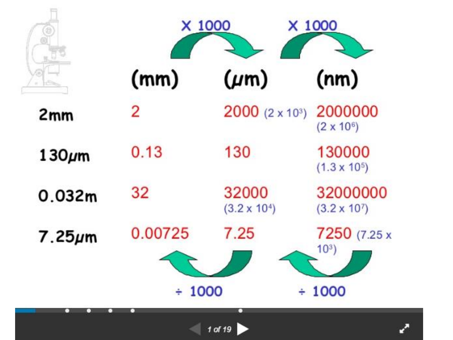
Scientific notation, exemplified by expressions like 2.9 x 10⁻⁶ meters, serves as the backbone of precision in biological sciences, enabling researchers to quantify structures ranging from submicroscopic organelles to macroscopic organisms with unparalleled accuracy. This system transcends mere mathematical convenience—it reflects the inherent scale of life, where dimensions often span orders of magnitude from nanometers (e.g., DNA strands) to kilometers (e.g., migratory patterns of whales). The notation 2.9 x 10 (with an implied exponent) standardizes communication across disciplines, ensuring consistency in experiments, publications, and collaborative research. Without it, fields like microbiology, cell biology, and evolutionary biology would struggle to reconcile the vast disparities in size, function, and spatial organization of living systems. The adoption of scientific notation in biology was not merely an administrative reform but a revolution in observational capability. As microscopes evolved from Leeuwenhoek’s rudimentary lenses to electron microscopes capable of resolving atomic structures, the need for a universal language to describe these discoveries became critical. Today, notations like 2.9 x 10⁻³ meters (2.9 millimeters) or 2.9 x 10⁻⁶ meters (2.9 micrometers) are ubiquitous, yet their interpretation demands both mathematical literacy and contextual understanding of biological scales. Missteps in translating these notations—such as confusing 10⁻⁶ (micrometers) with 10⁻³ (millimeters)—can lead to erroneous conclusions in studies of cellular pathology, drug delivery systems, or ecological interactions.
Mathematical and Scientific Foundations of "2.9 x 10" Notation
 Scientific notation, formally defined as a x 10ⁿ, where 1 ≤ a
micro-
(10⁻⁶), milli- (10⁻³), and nano- (10⁻⁹) correspond directly to powers of ten. For example:The elegance of this system lies in its ability to compress complexity. A human red blood cell, measuring roughly 7 x 10⁻⁶ meters (7 µm), can be compared instantly to a 100 µm-long Caenorhabditis elegans nematode without cumbersome decimal notation. This efficiency is particularly vital in multi-scale biological models, where researchers integrate data from molecular interactions (nanometers) to organismal behavior (meters).
Scientific notation is not just a tool for brevity; it is a cognitive scaffold that allows biologists to navigate the logarithmic scale of life, reducing the risk of errors in transcription, calculation, and interpretation.
Real-World Biological Applications of "2.9 x 10" Measurements
 The relevance of 2.9 x 10-style notations extends across biological subfields, where precise measurements dictate experimental design, diagnostic accuracy, and theoretical frameworks. Below are critical examples where such notations define the boundaries of scientific inquiry:
In biological research, a misinterpretation of 2.9 x 10⁻⁶ meters as 2.9 x 10⁻³ meters could lead to errors in drug dosage calculations for nanoparticles, cell culture conditions, or ecological niche modeling—highlighting the notation’s role as both a scientific language and a precision tool.
Comparative Table: Biological Structures and Their Scientific Notation
Understanding the context of 2.9 x 10-style measurements requires a cross-disciplinary perspective. The following table synthesizes key biological structures, their notational representations, and the tools used to quantify them:
| Measurement Notation | Equivalent Value | Biological Context | Measurement Tool Used |
|---|---|---|---|
| 2.9 x 10⁻⁹ m | 2.9 nanometers (nm) | Width of a DNA double helix or a single protein alpha-helix | Atomic Force Microscope (AFM), Cryo-Electron Microscopy |
| 2.9 x 10⁻⁸ m | 29 nanometers (nm) | Diameter of a ribosome (70S in prokaryotes) | Transmission Electron Microscope (TEM) |
| 2.9 x 10⁻⁷ m | 290 nanometers (nm) | Wavelength of ultraviolet light absorbed by DNA (damaging radiation) | Spectrophotometer, UV-Vis Spectroscopy |
| 2.9 x 10⁻⁶ m | 2.9 micrometers (µm) | Diameter of a red blood cell (human erythrocyte) | Light Microscope (with oil immersion, ~1.2 µm resolution) |
| 2.9 x 10⁻⁵ m | 29 micrometers (µm) | Length of a typical human sperm cell | Phase-Contrast Microscope, Differential Interference Contrast (DIC) |
| 2.9 x 10⁻⁴ m | 0.29 millimeters (mm) | Width of a fruit fly’s compound eye facet | Scanning Electron Microscope (SEM) |
| 2.9 x 10⁻³ m | 2.9 millimeters (mm
Microscopic Marvels: Organisms and Structures Within the 2.9 x 10⁻⁶ to 2.9 x 10⁻³ Meter SpectrumThe microscopic world thrives within a narrow yet critical range of measurements, where organisms and structures often fall between 2.9 x 10⁻⁶ meters (2.9 micrometers) and 2.9 x 10⁻³ meters (2.9 millimeters). This range bridges the gap between visibility under a standard light microscope and the need for advanced imaging techniques, such as electron microscopy. Organisms within this spectrum exhibit unique biological adaptations, from prokaryotic simplicity to eukaryotic complexity, while their sizes are dictated by evolutionary constraints, environmental pressures, and physiological scaling laws. Understanding these measurements is not merely an academic exercise—it illuminates critical insights into metabolism, disease mechanisms, and even the limits of life itself. The "2.9 x 10" notation becomes particularly significant when discussing structures that lie at the cusp of observational technology. For instance, a paramecium (≈2.9 x 10⁻⁴ m) is visible under a light microscope, while a ribosome (≈2.9 x 10⁻⁸ m) requires electron microscopy to resolve. This section explores ten key organisms and structures within this range, their measurement techniques, and the scientific implications of their sizes. Additionally, it examines exceptions that challenge the typical boundaries, environmental influences on scaling, and case studies where precise measurements revolutionized biological understanding.Categorization of Organisms and Structures by Size and TypeOrganisms within the 2.9 x 10⁻⁶ to 2.9 x 10⁻³ meter range span diverse biological kingdoms, from bacteria to multicellular structures. Their sizes are often expressed in scientific notation to convey precision, especially when discussing limits of microscopic resolution. Below is a categorized breakdown, emphasizing how each group interacts with measurement techniques and biological function.Prokaryotes: The Tiny Architects of LifeProkaryotes, lacking a nucleus and membrane-bound organelles, dominate the lower end of the 2.9 x 10 spectrum. Their sizes are constrained by surface-area-to-volume ratios, nutrient uptake efficiency, and replication speed. Many prokaryotes fall within 2.9 x 10⁻⁶ to 2.9 x 10⁻⁵ meters, making them ideal candidates for electron microscopy. Below are three notable examples:Scientific Notation in Prokaryotes: The use of 2.9 x 10⁻⁶ m notation for E. coli highlights its proximity to the resolution limit of light microscopes (~2 x 10⁻⁶ m). Below this threshold, electron microscopy becomes indispensable. Eukaryotic Cells: Complexity Within Microscopic DimensionsEukaryotic cells, larger and more structurally complex than prokaryotes, often occupy the 2.9 x 10⁻⁵ to 2.9 x 10⁻⁴ meter range. Their sizes are influenced by the need to house organelles like mitochondria and nuclei while maintaining efficient transport mechanisms. Below are three eukaryotic cells whose measurements fall within this critical spectrum:Surface-Area-to-Volume Ratio: Eukaryotic cells like red blood cells optimize this ratio to balance nutrient uptake, waste removal, and structural integrity. Larger cells (e.g., Paramecium) require internal transport systems (e.g., cytoskeletal networks) to compensate for reduced efficiency. Cell Organelles: The Nanoscale Engines of LifeOrganelles operate at the 2.9 x 10⁻⁷ to 2.9 x 10⁻⁶ meter scale, where quantum mechanical effects and molecular interactions dominate. Their sizes are critical for enzymatic efficiency, protein synthesis, and energy production. Three key organelles within this range include:Resolution Limits: Organelles like ribosomes and mitochondrial cristae push the boundaries of light microscopy. The Abbe diffraction limit (≈2 x 10⁻⁷ m) necessitates electron microscopy or super-resolution techniques (e.g., STED microscopy) for detailed imaging. Multicellular Structures: Miniature Architectures at the Microscopic-Macroscopic InterfaceMulticellular structures near the upper limit of the 2.9 x 10⁻³ m range exhibit emergent properties that defy individual cell behavior. Their sizes are often dictated by developmental constraints and functional requirements, such as nutrient distribution or reproductive strategies. Examples include:The next time an organism measures 2.9 x 10 units crosses your path—whether in a lab report, a research paper, or a cutting-edge discovery—remember that behind those three simple symbols lies a universe of precision, history, and unanswered questions. This notation is not just a tool for scientists; it is the silent thread connecting the visible world to the microscopic frontier, where every decimal point could unlock new frontiers in medicine, ecology, or synthetic biology. As technology advances and our ability to measure shrinks further, the significance of "2.9 x 10" will only grow, reinforcing its place as a cornerstone of biological inquiry for generations to come. |
Leave a Comment
Comments are moderated before appearing. The data you submit is processed according to the Privacy Policy of Cloudpbx.