Mastering sequences when starting at first quadrant coordinates 3 7 moving 3 uni
Table of Contents
- Understanding Quadrants in Mathematical Sequences: Foundations and Applications
- Structural Breakdown of Mathematical Quadrants
- Comparative Analysis of Quadrant Characteristics
- Role of the First Quadrant as a Reference Point
- Real-World Analogies for Quadrant-Based Movement
- Decoding the Sequence Rule: Starting at (3,7) and Moving 3 Units Down in the First Quadrant
- Significance of the Starting Coordinate (3,7) in the First Quadrant
- Mathematical Implications of Moving 3 Units Down
- Step-by-Step Generation of Subsequent Coordinates
- Comparison of Coordinates After Each Movement
- Clarifying Potential Misinterpretations of the Movement Rule
- Visualizing the Sequence Path: Graphs, Diagrams, and Interactive Elements in Quadrant-Based Movement
- Constructing a 2D Graph for Sequence Path Visualization
- Designing an Interactive HTML/JavaScript Visualization
- Creating Static Diagrams for Sequence Representation
Navigating mathematical sequences begins with a fundamental question: what happens when you anchor a path at coordinates 3,7 in the first quadrant and instruct it to move downward? This seemingly simple rule triggers a cascade of geometric precision and algebraic logic, revealing how quadrants govern the behavior of sequences in coordinate systems. Beyond abstract theory, such movements underpin real-world applications from game development to GPS mapping, where directional accuracy determines outcomes.
The first quadrant, defined by positive x and y axes, serves as the cornerstone for plotting trajectories in two-dimensional space. Starting at (3,7) and executing a downward shift of 3 units doesn’t just alter coordinates—it initiates a predictable yet transformative journey across mathematical boundaries. Whether analyzing patterns in data visualization or designing interactive simulations, understanding this rule unlocks deeper insights into how sequences evolve under systematic constraints. The interplay between starting positions and directional commands forms the backbone of coordinate-based problem-solving.
Understanding Quadrants in Mathematical Sequences: Foundations and Applications
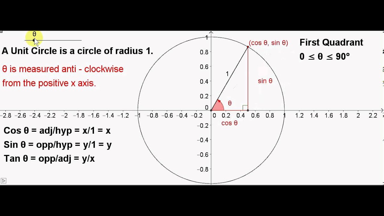
Mathematical quadrants serve as the structural backbone of coordinate systems, enabling precise representation of spatial relationships and sequential movements. Rooted in Cartesian geometry, quadrants divide a two-dimensional plane into four distinct regions, each defined by the intersection of the x-axis (horizontal) and y-axis (vertical). This segmentation is not merely theoretical; it underpins algorithms in computer science, navigation systems in aviation, and procedural generation in game design. The first quadrant, where both x and y coordinates are positive, acts as the reference point for defining movement and sequences, establishing a standardized framework for further exploration into negative territories. By mastering quadrant-based navigation, mathematicians, engineers, and developers gain the tools to model complex systems, from plotting trajectories in physics to designing interactive environments in virtual reality. The Cartesian plane’s quadrants create a systematic approach to sequencing, where each region dictates the sign and behavior of coordinates. Movement within these quadrants follows predictable patterns, influenced by the algebraic rules governing positive and negative values. For instance, transitioning from the first to the third quadrant involves crossing both axes, altering the sign of both x and y coordinates. This transition is critical in sequence generation, where each step may dictate a shift in quadrant, thereby modifying the properties of subsequent terms. Understanding these dynamics allows for the creation of adaptive algorithms, such as those used in robotics for pathfinding or in economics for modeling cyclical trends.
Structural Breakdown of Mathematical Quadrants
 Quadrants are defined by the perpendicular intersection of the x-axis and y-axis, dividing the plane into four distinct regions labeled counterclockwise from the first quadrant (I) to the fourth (IV). Each quadrant exhibits unique characteristics in terms of coordinate signs, movement directions, and practical applications. The first quadrant, bounded by the positive x-axis and positive y-axis, serves as the origin for most mathematical sequences due to its simplicity and intuitive alignment with real-world positive measurements. Adjacent quadrants extend this framework into negative territories, introducing complexities that challenge and expand problem-solving strategies.
The orientation of axes within each quadrant dictates the algebraic behavior of coordinates. For example:
Quadrants are defined by the perpendicular intersection of the x-axis and y-axis, dividing the plane into four distinct regions labeled counterclockwise from the first quadrant (I) to the fourth (IV). Each quadrant exhibits unique characteristics in terms of coordinate signs, movement directions, and practical applications. The first quadrant, bounded by the positive x-axis and positive y-axis, serves as the origin for most mathematical sequences due to its simplicity and intuitive alignment with real-world positive measurements. Adjacent quadrants extend this framework into negative territories, introducing complexities that challenge and expand problem-solving strategies.
The orientation of axes within each quadrant dictates the algebraic behavior of coordinates. For example:
Comparative Analysis of Quadrant Characteristics
The following table summarizes the defining features of each quadrant, including axis orientation, movement patterns, example coordinates, and common use cases. This comparative structure highlights how quadrants differ in their mathematical behavior and practical applications, reinforcing their role in sequence-based problems.| Quadrant | Axis Orientation | Movement Patterns | Example Coordinates | Common Use Cases |
|---|---|---|---|---|
| I | x > 0, y > 0 | Right (+x), Up (+y) | (3, 7), (5, 10), (0.5, 2) |

|
| II | x < 0, y > 0 | Left (–x), Up (+y) | (–4, 6), (–1, 3), (–2.5, 8) |
|
| III | x < 0, y < 0 | Left (–x), Down (–y) | (–3, –5), (–7, –2), (–1.2, –4) |
|
| IV | x > 0, y < 0 | Right (+x), Down (–y) | (6, –3), (2, –8), (4.5, –1) |
|
Role of the First Quadrant as a Reference Point
The first quadrant’s dominance as a starting point in mathematical sequences stems from its alignment with intuitive, real-world measurements. In this region, both x and y coordinates are positive, eliminating the complexity of negative values and providing a clear, unobstructed space for initial calculations. This simplicity extends to visual representations, where graphs in Quadrant I are easier to interpret due to the absence of axis crossings or sign ambiguities. For instance, plotting a linear sequence like (1, 2), (2, 4), (3, 6) in Quadrant I reveals an immediate upward trend, whereas the same sequence in Quadrant III would appear as (–1, –2), (–2, –4), (–3, –6), obscuring the relationship between terms. The boundaries of the first quadrant are defined by the positive x-axis (y = 0) and positive y-axis (x = 0), creating a 90-degree sector where both coordinates increase simultaneously. Adjacent quadrants extend this framework by introducing negative values, but their definitions rely on the first quadrant’s foundational rules. For example, the second quadrant’s negative x-values are measured as a deviation from the positive x-axis of Quadrant I, while its positive y-values retain the upward orientation. This adjacency ensures continuity in mathematical operations, allowing sequences to transition smoothly between regions without disrupting algebraic integrity. In sequence generation, the first quadrant often serves as the "home" position, from which movements are defined. For example, a problem might instruct: "Begin at (3, 7) in Quadrant I and move 3 units down." The solution remains within Quadrant I because the y-coordinate decreases to 4, while the x-coordinate (3) remains unchanged. However, if the instruction were "move 5 units left," the new x-coordinate (–2) would shift the point to Quadrant II, demonstrating how the first quadrant’s reference role enables precise navigation across the entire plane.Real-World Analogies for Quadrant-Based Movement
Quadrant-based systems are ubiquitous in fields where spatial relationships dictate outcomes. Navigation provides a clear example: pilots use quadrants to plot flight paths relative to a starting point. Departing from anDecoding the Sequence Rule: Starting at (3,7) and Moving 3 Units Down in the First Quadrant
Understanding how sequences are generated in coordinate systems requires precision, particularly when defining starting points and movement rules. The sequence rule "start at (3,7) and move 3 units down" operates within the Cartesian plane’s first quadrant, where both x and y coordinates are positive. This rule establishes a structured progression that relies on the Cartesian axes for directionality. The first quadrant’s constraints—where x ≥ 0 and y > 0—ensure that movements like "down" strictly affect the y-coordinate while leaving the x-coordinate unchanged unless specified otherwise. This foundational rule serves as a template for more complex sequences, emphasizing the importance of clarity in defining movement directions to avoid ambiguity in coordinate transformations. The rule’s components—starting point and movement command—interact to define a linear progression along the y-axis. The starting coordinate (3,7) anchors the sequence, while the instruction "move 3 units down" dictates the transformation applied iteratively. This interaction forms the basis for generating subsequent coordinates, where each step adheres to the mathematical operation of decrementing the y-value while preserving the x-value. Such rules are critical in applications ranging from computer graphics to algorithmic pathfinding, where precise coordinate manipulation is essential.Significance of the Starting Coordinate (3,7) in the First Quadrant
The starting coordinate (3,7) holds dual importance in this sequence. First, its position in the first quadrant ensures both x (3) and y (7) are positive, aligning with the quadrant’s defining characteristics. The x-coordinate (3) represents the horizontal distance from the origin (0,0), while the y-coordinate (7) indicates vertical distance. This placement is arbitrary yet structured, as sequences can commence at any coordinate within the quadrant, provided the movement rule remains consistent. For instance, starting at (5,10) would yield a different sequence than (3,7), but the underlying principle—preserving x while modifying y—remains identical. The choice of (3,7) as a starting point demonstrates how sequences can be tailored to specific contexts, such as plotting data points in a graph or defining paths in a grid-based system. Its significance lies in its role as a reference for subsequent transformations, ensuring reproducibility and predictability in the sequence’s progression.Mathematical Implications of Moving 3 Units Down
The instruction "move 3 units down" translates to a vertical displacement along the y-axis, specifically a decrement in the y-coordinate. In mathematical terms, downward movement in the Cartesian plane corresponds to subtracting the movement units from the initial y-value. This operation is governed by the formula:New y-coordinate = Initial y-coordinate − Movement unitsFor the given rule, this becomes: New y-coordinate = 7 − 3 = 4. Thus, the new coordinate after the first movement is (3,4). This operation contrasts with other possible movements:
Step-by-Step Generation of Subsequent Coordinates
Generating the next five coordinates in the sequence requires iterative application of the movement rule. Each step involves decrementing the y-coordinate by 3 units while retaining the x-coordinate. Below is a procedural breakdown:Comparison of Coordinates After Each Movement
The following table summarizes the transformation at each step, including the original coordinates, movement direction, new coordinates, and the resulting quadrant:| Step | Original Coordinates | Movement Direction | New Coordinates | Quadrant of New Position |
|---|---|---|---|---|
| Initial | (3,7) | — | — | First Quadrant |
| 1 | (3,7) | 3 units down | (3,4) | First Quadrant |
| 2 | (3,4) | 3 units down | (3,1) | First Quadrant (boundary) |
| 3 | (3,1) | 3 units down | (3,−2) | Fourth Quadrant |
| 4 | (3,−2) | 3 units down | (3,−5) | Fourth Quadrant |
| 5 | (3,−5) | 3 units down | (3,−8) | Fourth Quadrant |
Clarifying Potential Misinterpretations of the Movement Rule
Ambiguity in movement rules can arise from imprecise language or misinterpretations of directional commands. For the rule "move 3 units down", two common misinterpretations warrant clarification: 1. Diagonal Movement: A misreading might suggest moving diagonally (e.g., down-left or down-right), which would alter both x and y coordinates. For example, moving diagonally down-left by 3 units could imply decrementing both x and y by 3, resulting in (0,4) from (3,7). However, the rule specifies strictly vertical movement, requiring only the y-coordinate to change. 2. Horizontal Movement: Another misinterpretation could involve moving horizontally (left or right) instead of vertically. For instance, moving 3 units left from (3,7) would yield (0,7), which contradicts theVisualizing the Sequence Path: Graphs, Diagrams, and Interactive Elements in Quadrant-Based Movement
Understanding mathematical sequences often benefits from visualization, especially when movement patterns are involved. A sequence starting at (3,7) in the first quadrant and moving 3 units down repeatedly creates a predictable yet visually distinct path. Constructing accurate graphs, interactive diagrams, and static representations not only clarifies the sequence’s behavior but also highlights how starting coordinates and movement rules influence trajectory. This section explores methods to plot such sequences, including 2D graph construction, interactive JavaScript-based visualization, and static diagram design, while emphasizing quadrant-specific behaviors and color-coding techniques for enhanced clarity.Constructing a 2D Graph for Sequence Path Visualization
A 2D Cartesian graph serves as the foundational tool for plotting sequences with directional movement. For a sequence starting at (3,7) and moving 3 units down in the first quadrant, the graph must clearly depict:| Q3 | Q4 |
|---|
Leave a Comment
Comments are moderated before appearing. The data you submit is processed according to the Privacy Policy of Cloudpbx.